import pandas as pd
import numpy as np
from IPython.display import display, HTML, Markdown
import ipywidgets as widgets
from ipywidgets.embed import embed_minimal_html, dependency_state
from matplotlib import pyplot as plt
import seaborn as sns
import humanize
import gettext
from babel import Locale
import imgkit
import warnings
import urllib
Для скачивания используется команда curl или wget
Описание данных и репозиторий:
https://github.com/owid/covid-19-data/tree/master/public/data/excess_mortality
Данные о населении:
https://raw.githubusercontent.com/owid/covid-19-data/master/public/data/latest/
!curl https://raw.githubusercontent.com/owid/covid-19-data/master/public/data/excess_mortality/excess_mortality.csv > excess_mortality.csv
% Total % Received % Xferd Average Speed Time Time Time Current Dload Upload Total Spent Left Speed 100 286k 100 286k 0 0 872k 0 --:--:-- --:--:-- --:--:-- 872k
!curl https://raw.githubusercontent.com/owid/covid-19-data/master/public/data/latest/owid-covid-latest.csv > owid-covid-latest.csv
% Total % Received % Xferd Average Speed Time Time Time Current Dload Upload Total Spent Left Speed 100 48171 100 48171 0 0 207k 0 --:--:-- --:--:-- --:--:-- 207k
!wget https://raw.githubusercontent.com/owid/covid-19-data/master/public/data/excess_mortality/excess_mortality.csv -O excess_mortality.csv
--2020-12-25 14:20:06-- https://raw.githubusercontent.com/owid/covid-19-data/master/public/data/excess_mortality/excess_mortality.csv Распознаётся raw.githubusercontent.com (raw.githubusercontent.com)… 151.101.36.133 Подключение к raw.githubusercontent.com (raw.githubusercontent.com)|151.101.36.133|:443... соединение установлено. HTTP-запрос отправлен. Ожидание ответа… 200 OK Длина: 292888 (286K) [text/plain] Сохранение в: «excess_mortality.csv» excess_mortality.cs 100%[===================>] 286,02K --.-KB/s за 0,1s 2020-12-25 14:20:06 (2,02 MB/s) - «excess_mortality.csv» сохранён [292888/292888]
!wget https://raw.githubusercontent.com/owid/covid-19-data/master/public/data/latest/owid-covid-latest.csv -O owid-covid-latest.csv
--2020-12-25 14:20:06-- https://raw.githubusercontent.com/owid/covid-19-data/master/public/data/latest/owid-covid-latest.csv Распознаётся raw.githubusercontent.com (raw.githubusercontent.com)… 151.101.36.133 Подключение к raw.githubusercontent.com (raw.githubusercontent.com)|151.101.36.133|:443... соединение установлено. HTTP-запрос отправлен. Ожидание ответа… 200 OK Длина: 48171 (47K) [text/plain] Сохранение в: «owid-covid-latest.csv» owid-covid-latest.c 100%[===================>] 47,04K --.-KB/s за 0,04s 2020-12-25 14:20:07 (1,03 MB/s) - «owid-covid-latest.csv» сохранён [48171/48171]
df = pd.read_csv('excess_mortality.csv')
df_population = pd.read_csv('owid-covid-latest.csv')
df.head()
location | date | p_scores_all_ages | p_scores_15_64 | p_scores_65_74 | p_scores_75_84 | p_scores_85plus | deaths_2020_all_ages | avg_deaths_2015_2019 | deaths_2015_all_ages | ... | deaths_2012_all_ages | deaths_2013_all_ages | deaths_2014_all_ages | Week | Cumulative excess deaths, all ages | Excess mortality cumulative P-scores, ages 15–64 | Excess mortality cumulative P-scores, ages 65–74 | Excess mortality cumulative P-scores, ages 75–84 | Excess mortality cumulative P-scores, ages 85+ | Excess mortality cumulative P-scores, all ages | |
---|---|---|---|---|---|---|---|---|---|---|---|---|---|---|---|---|---|---|---|---|---|
0 | Austria | 2020-01-05 | -10.95 | -5.42 | -23.21 | -5.30 | -11.17 | 1611.0 | 1809.0 | 1704.0 | ... | 1574.0 | 1637.0 | 1549.0 | 1 | -198.0 | -5.42 | -23.21 | -5.30 | -11.17 | -10.95 |
1 | Austria | 2020-01-12 | -8.35 | -1.45 | -5.43 | -5.30 | -13.40 | 1702.0 | 1857.0 | 1768.0 | ... | 1563.0 | 1659.0 | 1543.0 | 2 | -353.0 | -3.43 | -14.51 | -5.30 | -12.32 | -9.63 |
2 | Austria | 2020-01-19 | 0.59 | -7.32 | -1.09 | 9.77 | -2.91 | 1797.0 | 1786.4 | 1837.0 | ... | 1586.0 | 1612.0 | 1578.0 | 3 | -342.4 | -4.75 | -10.11 | -0.44 | -9.24 | -6.28 |
3 | Austria | 2020-01-26 | 1.89 | 14.20 | -5.11 | 10.18 | -4.88 | 1780.0 | 1747.0 | 1792.0 | ... | 1595.0 | 1584.0 | 1463.0 | 4 | -309.4 | -0.15 | -8.89 | 2.07 | -8.17 | -4.30 |
4 | Austria | 2020-02-02 | 7.06 | -5.91 | -0.22 | 19.98 | 5.79 | 1947.0 | 1818.6 | 1837.0 | ... | 1545.0 | 1752.0 | 1574.0 | 5 | -181.0 | -1.33 | -7.16 | 5.63 | -5.35 | -2.01 |
5 rows × 26 columns
df.location.unique()
array(['Austria', 'Belgium', 'Bulgaria', 'Canada', 'Chile', 'Croatia', 'Czechia', 'Denmark', 'England & Wales', 'Estonia', 'Finland', 'France', 'Germany', 'Greece', 'Hungary', 'Iceland', 'Israel', 'Italy', 'Latvia', 'Lithuania', 'Luxembourg', 'Netherlands', 'New Zealand', 'Northern Ireland', 'Norway', 'Poland', 'Portugal', 'Scotland', 'Slovakia', 'Slovenia', 'South Korea', 'Spain', 'Sweden', 'Switzerland', 'Taiwan', 'United Kingdom', 'United States'], dtype=object)
df.columns
Index(['location', 'date', 'p_scores_all_ages', 'p_scores_15_64', 'p_scores_65_74', 'p_scores_75_84', 'p_scores_85plus', 'deaths_2020_all_ages', 'avg_deaths_2015_2019', 'deaths_2015_all_ages', 'deaths_2016_all_ages', 'deaths_2017_all_ages', 'deaths_2018_all_ages', 'deaths_2019_all_ages', 'deaths_2010_all_ages', 'deaths_2011_all_ages', 'deaths_2012_all_ages', 'deaths_2013_all_ages', 'deaths_2014_all_ages', 'Week', 'Cumulative excess deaths, all ages', 'Excess mortality cumulative P-scores, ages 15–64', 'Excess mortality cumulative P-scores, ages 65–74', 'Excess mortality cumulative P-scores, ages 75–84', 'Excess mortality cumulative P-scores, ages 85+', 'Excess mortality cumulative P-scores, all ages'], dtype='object')
if False:
df_population.columns
columns = ['iso_code', 'continent', 'location', 'total_cases', 'population', 'population_density']
with pd.option_context('display.float_format', '{: .2f}'.format):
display(df_population[columns])
country = 'Sweden'
dfc =df[df.location==country]
# dfc
df_messages = pd.read_csv('locale/ru_RU/LC_MESSAGES/messages.csv')
def plot_deaths(df, country='Sweden', ax=None):
df = df[df.location==country]
if ax is None:
fig, ax = plt.subplots(figsize=(10, 8))
sns.relplot(data=df, x='Week', y='deaths_2020_all_ages', ax=ax, kind="line", color='red', label='2020')
ax.set_title(f'Deaths by week, {country}')
ax.legend()
plt.close()
sns.relplot(data=df, x='Week', y='avg_deaths_2015_2019', ax=ax, kind="line", color='black', label='average 2015-2019')
ax.legend()
ax.set_ylim(ymin=0)
plt.close()
df_deaths = agregate_by_years(df)
sns.relplot(x="Week", y="deaths", kind="line", ci="sd", data=df_deaths, ax=ax, label='average 2010-2019 (with std)')
ax.legend()
plt.close()
def plot_cumsum(df, country='Sweden', ax=None):
df = df[df.location==country]
if ax is None:
fig, ax = plt.subplots(figsize=(10, 8))
sns.relplot(data=df, x='Week', y='Cumulative excess deaths, all ages', ax=ax, kind="line")
ax.set_title(f'excess mortality by week, {country}')
plt.close()
def report(df, country='Sweden', display=True):
df = df[df.location==country]
cumsum = df['Cumulative excess deaths, all ages']
available = cumsum.notnull()
cumsum = cumsum[available]
d = {}
d['location'] = country
d['Weeks'] = len(cumsum)
deaths = df.avg_deaths_2015_2019[available].sum()
deaths2020 = df.deaths_2020_all_ages[available].sum()
d['deaths avg'] = deaths
d['deaths 2020'] = deaths2020
d['delta'] = deaths2020 - deaths
if len(cumsum) > 0:
d['comsum last'] = cumsum.values[-1]
d['excess'] = (deaths2020 - deaths) / deaths
population = df_population[df_population.location==country]
if len(population) != 1:
print(country, 'Population data is not available')
else:
d['population'] = int(population.iloc[0]['population'])
d['excess per population'] = d['delta'] / d['population']
d['deaths avg per population'] = d['deaths avg'] / d['population']
if display:
display_dict(d)
return d
else:
return d
def agregate_by_years(dfc):
df_deaths = []
for year in range(2010, 2020):
key = f'deaths_{year}_all_ages'
df_item = dfc[['date', 'Week']]
df_item = df_item.assign(year=key, deaths=dfc[key])
df_deaths.append(df_item)
df_deaths = pd.concat(df_deaths, axis=0)
df_deaths = df_deaths.reset_index(drop=True)
return df_deaths
def dict_to_html(d):
d2 = {}
for k, v in d.items():
if isinstance(v, (int, float)):
v = humanize.intcomma(v)
d2[k] = v
d = d2
dfr = pd.DataFrame(d.values(), index=d.keys())
with pd.option_context('display.float_format', '{: .2f}'.format):
res = dfr.to_html(header=False)
return res
def display_dict(d):
html = dict_to_html(d)
display(HTML(html))
def plot_and_report(df, country='Sweden'):
fig, axes = plt.subplots(figsize=(20, 8), ncols=2)
fig.suptitle(f'{country}')
plot_deaths(df, country, ax=axes[0])
plot_cumsum(df, country, ax=axes[1])
fn = f'images/{country}.png'
fig.savefig(fn)
d = report(df, country)
html = dict_to_html(d)
fn = f'images/{country}_report.png'
imgkit.from_string(html, fn, )
plot_and_report(df)
location | Sweden |
---|---|
Weeks | 48 |
deaths avg | 81,423.4 |
deaths 2020 | 85,567.0 |
delta | 4,143.600000000006 |
comsum last | 4,143.6 |
excess | 0.05088954772215366 |
population | 10,099,270 |
excess per population | 0.0004102870801552989 |
deaths avg per population | 0.008062305493367342 |
Loading page (1/2) Rendering (2/2) Done
plot_and_report(df, country='Norway')
location | Norway |
---|---|
Weeks | 47 |
deaths avg | 36,427.000000000015 |
deaths 2020 | 36,185.0 |
delta | -242.00000000001455 |
comsum last | -242.0 |
excess | -0.006643423833969706 |
population | 5,421,242 |
excess per population | -4.4639217360157424e-05 |
deaths avg per population | 0.0067193089701585015 |
Loading page (1/2) Rendering (2/2) Done
plot_and_report(df, country='Finland')
location | Finland |
---|---|
Weeks | 47 |
deaths avg | 48,132.80000000001 |
deaths 2020 | 49,333.0 |
delta | 1,200.1999999999898 |
comsum last | 1,200.2 |
excess | 0.024935179337166952 |
population | 5,540,718 |
excess per population | 0.00021661452540988187 |
deaths avg per population | 0.008687105173011874 |
Loading page (1/2) Rendering (2/2) Done
plot_and_report(df, country='United States')
location | United States |
---|---|
Weeks | 46 |
deaths avg | 2,446,576.0000000005 |
deaths 2020 | 2,836,704.0 |
delta | 390,127.99999999953 |
comsum last | 390,128.0 |
excess | 0.15945877013426088 |
population | 331,002,647 |
excess per population | 0.0011786250156482873 |
deaths avg per population | 0.00739140916900281 |
Loading page (1/2) Rendering (2/2) Done
plot_and_report(df, 'Lithuania')
location | Lithuania |
---|---|
Weeks | 49 |
deaths avg | 37,673.6 |
deaths 2020 | 38,665.0 |
delta | 991.4000000000015 |
comsum last | 991.4 |
excess | 0.02631551006540393 |
population | 2,722,291 |
excess per population | 0.0003641785540193908 |
deaths avg per population | 0.013838931987799981 |
Loading page (1/2) Rendering (2/2) Done
plot_and_report(df, 'Latvia')
location | Latvia |
---|---|
Weeks | 50 |
deaths avg | 27,200.2 |
deaths 2020 | 26,660.0 |
delta | -540.2000000000007 |
comsum last | -540.2 |
excess | -0.019860148087146444 |
population | 1,886,202 |
excess per population | -0.00028639562464677733 |
deaths avg per population | 0.014420618788443655 |
Loading page (1/2) Rendering (2/2) Done
if False:
for country in df.location.unique():
try:
plot_and_report(df, country)
except:
print(country)
if False:
html = ''
for country in selected:
url = urllib.parse.quote(f'{country}.png')
url = f"https://normalized2.github.io/covid/excess_mortality/images/{url}"
html += f'<a href="{url}">{country}</a> <br />\n'
display(HTML(html))
with warnings.catch_warnings():
warnings.simplefilter('ignore')
df_compare = pd.DataFrame([report(df, country, display=False) for country in df.location.unique()])
df_compare.to_csv('report.csv', index=False)
df_compare = df_compare.dropna()
# df_compare = df_compare[df_compare.location.isin(selected)]
# df_compare
selected = ['United States', 'Finland', 'Sweden', 'Norway', 'Latvia', 'Lithuania', 'Spain', 'Germany', 'Estonia']
df_compare[df_compare.location.isin(selected)]
England & Wales Population data is not available Northern Ireland Population data is not available Scotland Population data is not available
location | Weeks | deaths avg | deaths 2020 | delta | comsum last | excess | population | excess per population | deaths avg per population | |
---|---|---|---|---|---|---|---|---|---|---|
9 | Estonia | 50 | 14779.2 | 15100.0 | 320.8 | 320.8 | 0.021706 | 1326539.0 | 0.000242 | 0.011141 |
10 | Finland | 47 | 48132.8 | 49333.0 | 1200.2 | 1200.2 | 0.024935 | 5540718.0 | 0.000217 | 0.008687 |
12 | Germany | 47 | 838136.0 | 855309.0 | 17173.0 | 17173.0 | 0.020490 | 83783945.0 | 0.000205 | 0.010004 |
18 | Latvia | 50 | 27200.2 | 26660.0 | -540.2 | -540.2 | -0.019860 | 1886202.0 | -0.000286 | 0.014421 |
19 | Lithuania | 49 | 37673.6 | 38665.0 | 991.4 | 991.4 | 0.026316 | 2722291.0 | 0.000364 | 0.013839 |
24 | Norway | 47 | 36427.0 | 36185.0 | -242.0 | -242.0 | -0.006643 | 5421242.0 | -0.000045 | 0.006719 |
31 | Spain | 48 | 382508.8 | 453502.0 | 70993.2 | 70993.2 | 0.185599 | 46754783.0 | 0.001518 | 0.008181 |
32 | Sweden | 48 | 81423.4 | 85567.0 | 4143.6 | 4143.6 | 0.050890 | 10099270.0 | 0.000410 | 0.008062 |
36 | United States | 46 | 2446576.0 | 2836704.0 | 390128.0 | 390128.0 | 0.159459 | 331002647.0 | 0.001179 | 0.007391 |
def compare(data=df_compare, y='excess', select=selected, title=None):
data=data[data.location.isin(select)]
fig, ax = plt.subplots(figsize=(10, 6))
sns.barplot(x="location", y=y, data=data, ax=ax)
if title is None:
title = y
ax.set_title(title)
#plt.close()
fig.savefig(f'images/compare_{y}.png')
pass
compare(data=df_compare, y='excess', select=selected, title='Превышение смертей относительно среднего числа смертей за 2015-2019 года\n')
compare(data=df_compare, y='excess per population', select=selected, title='Превышение смертности, превышение числа смертей относительно численности населения')
compare(data=df_compare, y='deaths avg per population', select=selected, title='Cредняя смертность за 2015-2019 года')
compare(data=df_compare, y='Weeks', select=selected)
Week - количество недель за которые доступны данные
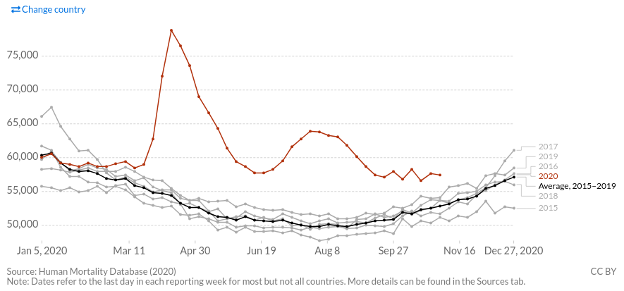
excess - превышение смертей относительно среднего числа смертей за 2015-2019 года, за доступное число недель
excess per population - превышение смертности, превышение числа смертей относительно численности населения, за доступное число недель
deaths avg per population - средняя смертность за 2015-2019 года, за доступное число недель
Допустим, средняя продолжительность жизни составляет 100 лет.
И предположим, что в устойчивой популяции рождается столько же сколько умирает. Тогда смертность будет в среднем 1 из 100, умирает 10 человек на каждую 1000.
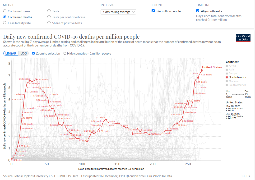
В Литве примерно 14 на тысячу, в США примерно 7 на тысячу. См. соотв. рис. выше.
Что означает, что превышение смертности в США равно 0.15 (относительно среднего числа смертей за 2015-2019 года)? Это значит, что вместо 10 человек в год на тысячу умерло на 15% больше. То есть 11,5.
И если судить субъективно только по своему окружению и по знакомым, то такое увеличение смертности практически незаметно.
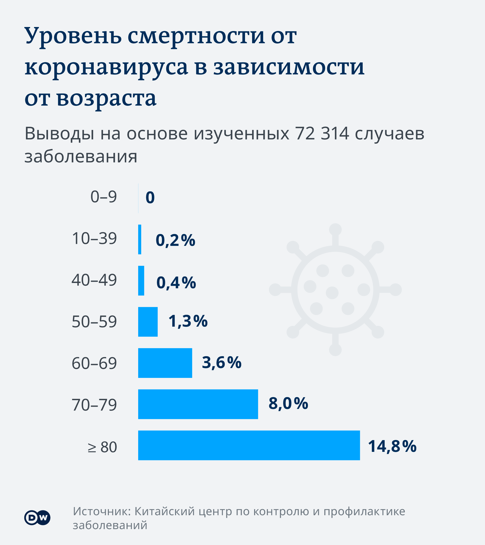
Особенно среди детей и молодых.
В соответствии с возрастным распределением летальности.
Например, среди московской епархии за 2020 год умерло почти в три раза больше чем в прошлом.
С другой стороны если в среднем за год умирало 2,5 миллиона человек, то увеличение смертности на 15% означает на 375 тысяч больше умерло. Не мало. Так же нужно учитывать запаздывание данных о превышении смертности на несколько недель. Ср рис 1 с рис 2
Средняя смертность за январь-октябрь 2020 складывается в основном за счет первой волны в марте-апреле, примерно два месяца. А так как ноябрь-декабрь-январь-февраль будет нелегким, то можно предположить (в зависимости от страны), что текущие оценки по превышению смертность к марту удвоятся или утроятся. За сезон 2020-03 - 2021-02.
Как видно, данные о смертности можно использовать в двух вариантах:
"Ерунда, вместо 10 человек умерло всего лишь на 1,5 человека больше, обычный грипп" В этом варианте не учитывается
"Вау, умерло на 375 тысяч больше"
Третий вариант, переболеем все за 12 месяцев без вакцины. Если принять во внимание, что данные о летальности около 2-4%, а в Москве, например, 2,2% -4,4%. Предположим, что за 12 месяцев переболеют 50%, тогда к фоновому уровню смертности 1 из 100 добавится еще 1-2 из 100, и превышение смертности достигнет 100-200%, в среднем за эти 12 месяцев.
Существенная циркуляция в обществе первого варианта приводит большим рискам, что получится третий. Насколько потеряет экономика судить не берусь. А если понимать опасность и не пренебрегать ею, то возможно удастся не доводить до существенных потерь. А при быстрой ликвидации вспышки, и как следствие снятия мер, экономика начала бы уже восстанавливаться.
Как сказать "Спасибо" источнику данных
https://ourworldindata.org/donate